Getting Onboard with Excel Spreadsheets and Functions
Open Workbook| Spreadsheet| Ribbon| Grid| Status Bar| Select Data| Enter Data| Save Workbook
Excel is a powerful spreadsheet tool for organizing and analyzing data. It is useful for many levels of data needs from simple calculations and keeping track of information to more complex data analysis and graphical displays. Spreadsheets reside in workbooks, which is kind of like a folder with individual documents inside.
Open a Workbook
Icons for Microsoft Excel have changed over the various versions of Excel, but the familiar green and white theme has remained a constant. You can find the Excel icon on your desktop or via the start menu on your computer. Click on this icon and select Blank Workbook.
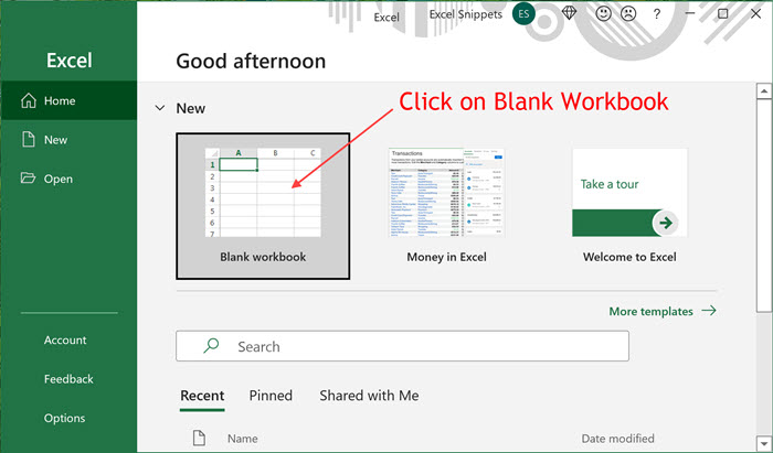
You have now opened a new blank workbook.
Tip: Workbook size limitations. A new workbook opens with only one sheet, but users can add up to 255 spreadsheets before needing to save the workbook. After that, you can add as many Excel sheets as your computer memory will accommodate.
Spreadsheet Structure
The key to using spreadsheets is understanding their fundamental structure, which comprises a
- Quick Access Bar
- - often used commands
- Ribbon
- - command groups
- Grid
- - area to enter and operate on data
- Status Bar
- - quick summary statistics
Below is a spreadsheet showing the basic layout.
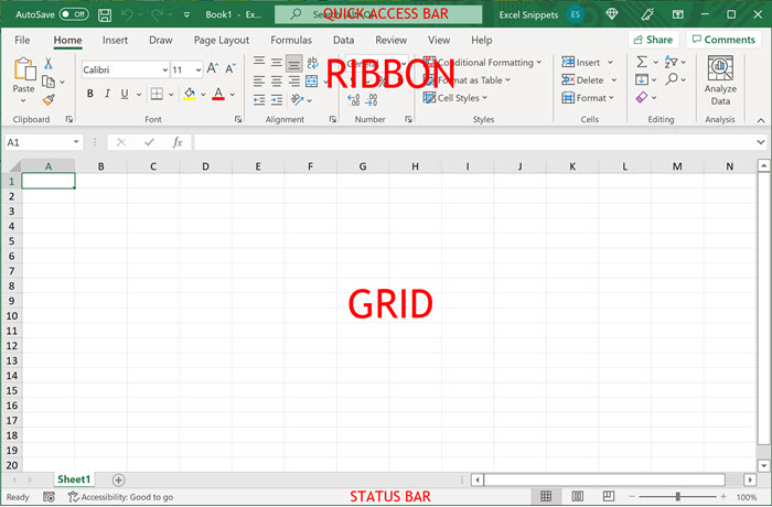
The main body of the grid are cells arranged in columns and rows. Columns are designated by letters, while rows by numbers. Above the grid is the Ribbon. Here, various commands can be accessed to operate on the data, save the workbook, and perform other actions. Select commands that are used more often than others appear in the Quick Access Bar, which can be customized by the user. When data is added to a worksheet, the user may select cells to see quick summary statistics displayed in the status bar area.
Excel Ribbon Layout
Below is the ribbon for the Home Tab. Available tabs appear as menu items at the top of the ribbon. The selected tab is underlined. It can be changed by selecting another menu item.
Beneath the menu area are Action Groups. The Home tab action groups are: Clipboard, Font, Alignment, Number, Styles, Cells, Editing, and Analyze Data. Earlier versions of Excel did not include this latter item as a default.
Within each action group are commands to modify or interact with data stored in the grid. In the action group titled Font, the font style and size may be changed from the default (Calibri and 11). Text color may also be changed, highlighted, emboldened, italicized or underlined. These are all visible in the Font group in the above figure, but additional font commands may be accessed by clicking on the small square with an arrow inside in the lower right-hand corner of the group area.
Some of the action groups have been collapsed because of space limitations, e.g. Cells. They can be accessed by clicking the down-pointing arrow beneath the group name. By expanding the spreadsheet window to a full-screen view, commands within these groups will become visible.

Grid Layout
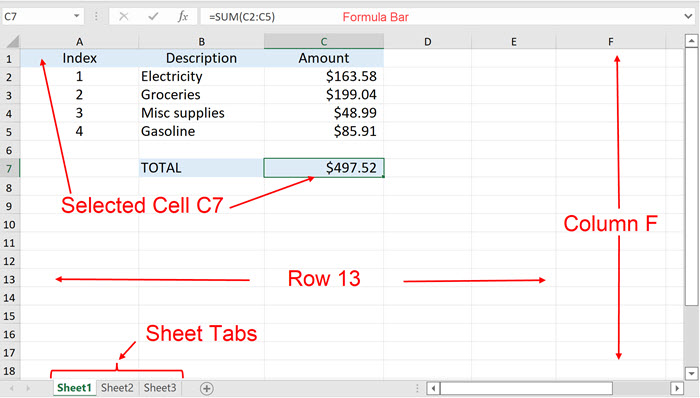
The main body of the grid is comprised of cells arranged in columns and rows. Just above is a window showing which cell in the grid has been selected. In this example cell C7 has been selected. Next to that window is the Formula Bar, which shows the content of the selected cell. Here the content is "=sum(C2:C5)."
Status Bar
When data is added to a worksheet, the user may select cells to see quick summary statistics displayed in the status bar area. More on this below.
Select Data in a Worksheet
Data may be stored in the cells of the grid. In cells in column A below are data in rows 1-4 and in column B in rows 1-6. The data in B2 is "Data item 2." Cells are referenced by adjoining the column letter and row number (CR). Data can be numerical or character. Different data types can be placed in the same column and columns do not need to have the same number of rows occupied, as shown here.
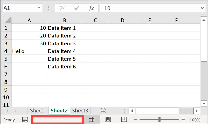
Open an Excel workbook and enter the data as shown here. Click on the cell in row 1, column A (cell A1). Then drag your cursor to select the area occupied by data as shown in the gray area below.
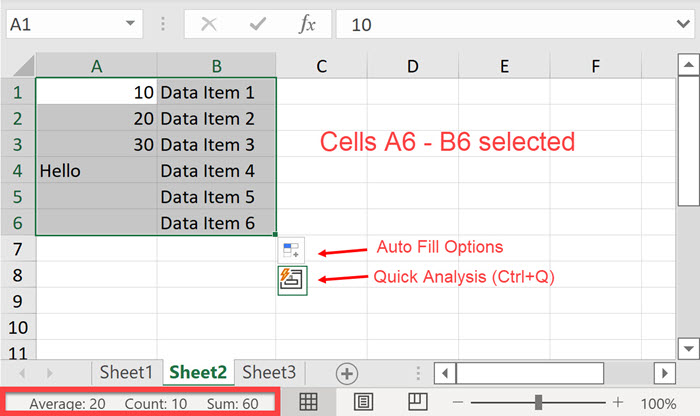
Notice the status bar in the grid with unselected cells above. Compare it with the one in the grid with data selected, where it gives a count of the number of cells with data in them (10 - 4 in column A and 6 in column B). It also totals the numeric data (60) and provides an average of the numeric data (20).
Enter Data into a Spreadsheet
Data may be stored in the cells of a worksheet several ways: manually by typing in the pieces of data, copy and paste from a variety of other document formats, or automated using Visual Basic for Applications (VBA).
Manually enter data into a spreadsheet:
Click on a cell, then type in a value. Press Enter to move to the next cell below this one or Tab to move to the next cell to the right. Done!
Copy and paste data into a spreadsheet:
You may copy data from other spreadsheets (worksheets) in this workbook or other workbooks, from Word documents, Pdf files, text files, and more. Once copied, select a cell in the spreadsheet where you wish the first piece of data to be entered. Click Paste in the ribbon or Right Click and select Paste to enter into the spreadsheet.
Visual Basic for Applications (VBA):
VBA is a built-in package that can automate data manipulation and calculations. The results may then stored in a spreadsheet or other document format. This method for entering data into a spreadsheet is covered in the VBA section in this website.
Save a Workbook
Now that you've created a workbook, you must save it if you wish to keep the contents. Select the File drop-down menu in the upper left-hand corner of the ribbon. Several options appear for saving the workbook: Save, Save As, or Save as Adobe PDF (if installed).
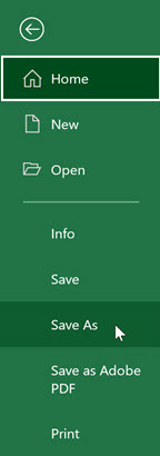
Since this is a new workbook, click on Save As, then select Browse. A window will appear that will allow you to save your workbook wherever you want on your computer. Navigate to the directory where you want to save the workbook.

By default, the first opened new workbook is called Book1.xlsx. You can change the filename to whatever you want by typing in a different name in the Filename Input Box. Then Click Save. Next time you modify this workbook, you need you can Click Save from the File menu to save it in the same location.
